Kick Google Scholar Up a Notch

Date: Published February 27, 2019; updated July 26, 2019 and February 4, 2020

(If you just want the code, go here.)

Maybe you’re applying for a job or going up for tenure, and are trying to demonstrate your research output in a unique way. In academia, the number of publications and citations are commonly used as indicators of productivity and influence - the hypothesis being that productive people are writing more papers and influential people are being cited more. The limitations of these metrics have long been noted, so I won’t belabor them here.

Nevertheless, some people in positions of power care about publications and citations, so we might as well show these metrics in a user-friendly manner. I like making graphs so I decided to put a couple simple graphs on the front page of my CV. Since one of the critiques of citation analysis is that it doesn’t account for different authorship roles, I wanted to separately show the data for papers on which I was the first author since I made the primary intellectual contribution for those studies. I don’t know if putting graphs in CVs is normal, but I was complimented on it during multiple job interviews, so in the end I’m glad I bothered.

Let’s set up our environment. We’ll use the scholar package to get the data, then rearrange it a bit with dplyr, reshape2, and stringr, and finally plot with ggplot2. So, let’s load some packages!

require(scholar)  # interface with google scholar
require(ggplot2)  # for plotting
require(dplyr)    # for data tidying
require(stringr)  # for working with string data

To get your data from Google Scholar, first you have to determine your Google Scholar ID. You can get this from the characters after the = in your Google Scholar URL. For instance, my Google Scholar URL is https://scholar.google.com/citations?user=XXIpO1YAAAAJ, so I know my ID is XXIpO1YAAAAJ.

me <- "XXIpO1YAAAAJ"

It’s easy to get a list of all your publications using the get_publications() function:

pubs_raw <- 
  scholar::get_publications(me)

While Google Scholar’s great, it makes some mistakes. For accuracy’s sake I’ll do a little cleaning up of this list. Specifically, I want to: (1) remove any non-journal articles such as theses; (2) remove anypre-prints that have not gone through peer review yet; and (3) adjust the years for an article that were published as preprints in 2019 but actually published in 2020 - Google Scholar puts these in the year the preprint was posted.

pubs <-
  pubs_raw %>% 
  # (1) remove theses; these don't have a year
  subset(is.finite(year)) %>% 
  # (2) get rid of preprints - all mine are on EarthArXiv
  subset(journal != "EarthArXiv")

# (3) update year - figure out the pubid by looking at the pubs_raw data frame
pubs$year[pubs$pubid == "fQNAKQ3IYiAC"] <- 2020

The author field has a comma-separated list of all the authors for each publication. Since I want to separately plot publications I first-authored, I need to isolate the first author for each paper:

pubs$first_author <- 
  # the 'author' column is a factor by default, so first convert to character
  pubs$author %>% 
  as.character() %>% 
  # split based on commas and grab the first author only
  strsplit(split="[,]") %>% 
  sapply(function(x) x[1])

# look at the results
pubs$first_author

##  [1] "SC Zipper"          "SC Zipper"          "SC Zipper"         
##  [4] "M Motew"            "SC Zipper"          "Y Kang"            
##  [7] "SC Zipper"          "SC Zipper"          "EG Booth"          
## [10] "J Qiu"              "P Lamontagne-Hallé" "J Qiu"             
## [13] "B Breyer"           "JE Vonk"            "LD Somers"         
## [16] "SC Zipper"          "SC Zipper"          "SC Zipper"         
## [19] "SC Zipper"          "J Qiu"              "SC Zipper"         
## [22] "C Zhang"            "SC Zipper"          "SC Zipper"         
## [25] "SC Zipper"          "M Motew"            "SC Zipper"         
## [28] "CL Tague"           "SC Zipper"          "X Chen"            
## [31] "KE Wallen"          "MA Nocco"

Uh-oh! I’m referred to as both “S Zipper” and “SC Zipper”. Fortunately, I don’t have any co-authors named Zipper, so I will claim anything including Zipper. If you have a more common last name, you might have to refine your search here.

my_name <- "Zipper"

pubs$first_author_me <-
  pubs$first_author %>% 
  stringr::str_detect(pattern = my_name)

We now have my publication history, and for every paper we know whether I am the first author or not. You can refine your search even more - for example, if you are a PI, you may want to create an additional category for publications by your students. You’d just need to remember their names.

Now, let’s work on the citations. The pubid field can be used to get annual citations for each of my publications. We’ll loop through all my papers, extract the citations by year, and put them into a big data frame. There’s probably a vectorized way to do this with apply but I didn’t bother because I don’t have that many papers.

for (i in 1:length(pubs$pubid)){
  # grab citations for this paper
  paper_cites <- 
    scholar::get_article_cite_history(id = me, 
                                      article = pubs$pubid[i])
  
  # make master data frame
  if (i == 1){
    all_cites <- paper_cites
  } else {
    all_cites <- rbind(all_cites, paper_cites)
  }
}

head(all_cites)

##   year cites        pubid
## 1 2017    13 cFHS6HbyZ2cC
## 2 2018    19 cFHS6HbyZ2cC
## 3 2019    31 cFHS6HbyZ2cC
## 4 2020     7 cFHS6HbyZ2cC
## 5 2017    14 3s1wT3WcHBgC
## 6 2018    15 3s1wT3WcHBgC

Now we know the annual citations for each paper, and can join it with pubs to add information about the first author.

all_cites <- 
  dplyr::left_join(all_cites,
                   pubs[, c("pubid", "first_author_me")],
                   by="pubid")

Let’s just re-arrange a bit to prepare for plotting.

# for the plots, we want annual sums
pubs_yr <-
  pubs %>% 
  dplyr::group_by(year, first_author_me) %>% 
  dplyr::summarize(number = n(),            # could use any field
                   metric = "Publications") # this will come in handy later
cites_yr <-
  all_cites %>% 
  dplyr::group_by(year, first_author_me) %>% 
  dplyr::summarize(number = sum(cites),
                   metric = "Citations")

# to make a faceted plot, we'll want to combine these into a single data frame
pubs_and_cites <- rbind(pubs_yr, cites_yr)

Finally - let’s make some graphs!

ggplot(pubs_and_cites, aes(x=factor(year), y=number, fill=first_author_me)) +
  geom_bar(stat="identity") +
  facet_wrap(~factor(metric, levels=c("Publications", "Citations")),
             scales = "free_y") +
  # everything below here is just aesthetics
  scale_x_discrete(name = "Year") +
  scale_y_continuous(name = "Number") +
  scale_fill_manual(name = "First Author", 
                    values = c("TRUE"="#e6194b", "FALSE"="#0082c8"),
                    labels = c("TRUE"="Zipper", "FALSE"="Other")) +
  theme_bw(base_size=12) +
  theme(panel.grid = element_blank(),
        strip.background = element_blank(),
        strip.text = element_text(size = 11, face="bold"),
        axis.title = element_text(size = 10, face="bold"),
        legend.title = element_text(size = 10, face="bold"),
        legend.position = c(0.01,0.99),
        legend.justification = c(0, 1))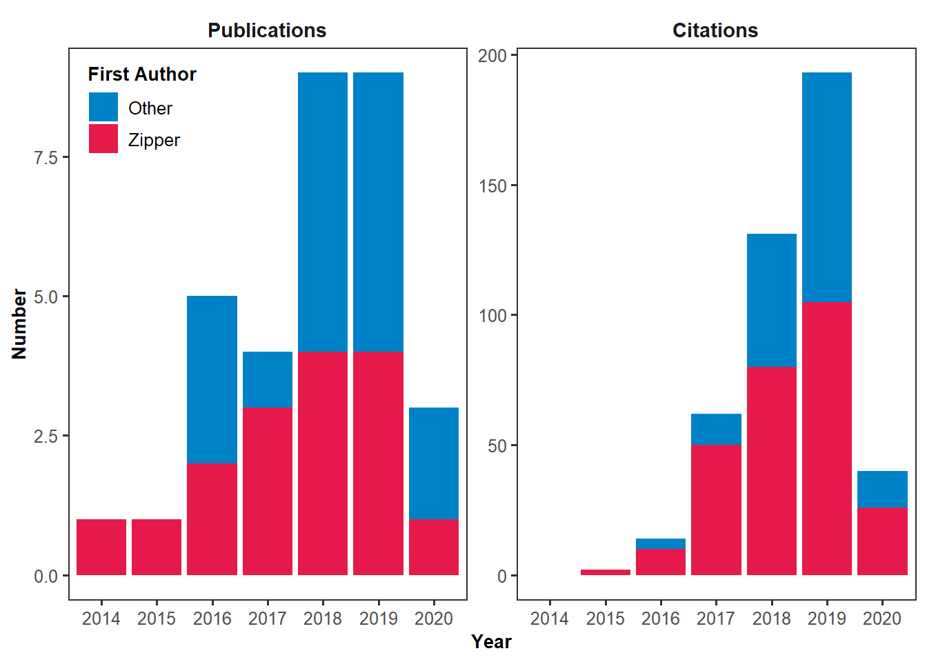

Voila! Now, you can add it to your CV, or just print it out and hang it on the wall above your bed (I don’t judge).